Astrometric precision horizons#
SHow the distance limits for the relative precision on parallaxes and proper motions. The plots produced are similar to figure 10 in Brown (2021) which is in turn based on figure 15 in Mateu et al. (2017).
import numpy as np
import matplotlib.pyplot as plt
from matplotlib import cm, colors

from pygaia.astrometry.constants import au_km_year_per_sec
from pygaia.errors.astrometric import (
    total_proper_motion_uncertainty,
    parallax_uncertainty,
)
from pygaia.photometry.transformations import gminic_from_vminic

plt.style.use("./agab.mplstyle")
Define absolute \(G\)-band magnitudes of a few tracer populations.#
Population |
Characteristic \(M_G\) |
|---|---|
Main sequence turn-off |
\(3.5\) |
Horizontal Branch |
\(0.5\) |
Tip of the Red Giant Branch |
\(-3.1\) |
For the TRGB the value of \(M_G\) is calculated from \((V-I_\mathrm{c})=1.5\) and \(M_{I_\mathrm{c}}=-4\).
gabs_msto = 3.5
gabs_hb = 0.5
vminic_trgb = 1.5
icabs_trgb = -4.0
gabs_trgb = gminic_from_vminic(vminic_trgb) + icabs_trgb
Relative proper motion uncertainty as a function of distance from the solar system barycentre#
The plot below is made for an estimate of typical tangential velocities which are calculated according to footnote 4 in Mateu et al. (2017).
“We assume that the radial velocity is on average \(v_r \sim v/\sqrt{3}\) and the total proper motion \(\mu \sim \sqrt{2/3}v\), where we assume \(v \sim v_\mathrm{e}/2\) and approximate the escape velocity as \(v_\mathrm{e} = v_\mathrm{c} \sqrt{2(1 − \ln(R_\mathrm{gal}/r_\mathrm{t}))}\), with \(v_\mathrm{c} = 200\) km s\(^{−1}\), \(r_\mathrm{t} = 200\) kpc and \(R_\mathrm{gal}\) the Galactocentric distance.”
gabs = np.linspace(-4, 4, 1000)
rhel = np.logspace(np.log10(10000), np.log10(200000), 1000)
mabsg, r = np.meshgrid(gabs, rhel)

mg = mabsg + 5 * np.log10(r) - 5
proper_motion_unc_dr4 = total_proper_motion_uncertainty(mg, release="dr4")
proper_motion_unc_dr5 = total_proper_motion_uncertainty(mg, release="dr5")

# Code lines below follow footnote 4 in Mateu et al. (2017)
vc = 200
rt = 200000
rsun = 8500
rGal = np.sqrt(r**2 + rsun**2)
ve = vc * np.sqrt(2 * (1 - np.log(rGal / rt)))

vtan = np.sqrt(2.0 / 3.0) * ve / 2
proper_motion = vtan / (r * au_km_year_per_sec) * 1.0e6
rel_pm_unc_dr4 = proper_motion_unc_dr4 / proper_motion
rel_pm_unc_dr5 = proper_motion_unc_dr5 / proper_motion

indices = np.where(mg > 20.7)
rel_pm_unc_dr4[indices] = np.nan
rel_pm_unc_dr5[indices] = np.nan

fig, ax = plt.subplots(1, 1, figsize=(15, 12))

for y in [gabs_trgb, gabs_hb, gabs_msto]:
    ax.plot(
        [rhel.min() / 1000, rhel.max() / 1000],
        [y, y],
        lw=2,
        ls="dotted",
        color="k",
        zorder=-1,
    )
ax.contour(rhel / 1000, gabs, mg.T, levels=[20.7], linestyles="dashdot", colors="gray")
ax.contour(
    rhel / 1000,
    gabs,
    rel_pm_unc_dr4.T,
    levels=[0.05, 0.5],
    colors=colors.to_rgba_array(cm.tab10.colors[0]),
    linestyles=["solid"],
)
ax.contour(
    rhel / 1000,
    gabs,
    rel_pm_unc_dr5.T,
    levels=[0.05, 0.5],
    colors=colors.to_rgba_array(cm.tab10.colors[1]),
    linestyles=["dashed"],
)
ax.invert_yaxis()
ax.set_xscale("log")
ax.set_xticks([10, 100], minor=False)
ax.set_xticklabels(["10", "100"], minor=False)
ax.set_xticks([20, 30, 40, 50, 60, 70, 80, 90, 200], minor=True)
ax.set_xticklabels(["20", "30", "40", "50", "60", "70", "80", "90", "200"], minor=True)
ax.set_xlabel(r"Barycentric distance [kpc]")
ax.set_ylabel(r"Absolute magnitude $M_G$ of tracer population")
ax.text(
    12, gabs_msto, "MSTO", ha="center", va="center", bbox=dict(facecolor="w", ec="w")
)
ax.text(12, gabs_hb, "HB", ha="center", va="center", bbox=dict(facecolor="w", ec="w"))
ax.text(
    12, gabs_trgb, "TRGB", ha="center", va="center", bbox=dict(facecolor="w", ec="w")
)

ax.text(65, 2.5, "Gaia survey limit", ha="center", rotation=35)
ax.text(40, 0.3, r"Gaia DR4: $\sigma_\mu/\mu<5$%", ha="center", rotation=55)
ax.text(30, 2.9, r"Gaia DR5: $\sigma_\mu/\mu<5$%", ha="center", rotation=49)
ax.text(97, 0.1, r"Gaia DR4: $\sigma_\mu/\mu<50$%", ha="center", rotation=52)
ax.text(130, 0.3, r"Gaia DR5: $\sigma_\mu/\mu<50$%", ha="center", rotation=52)

plt.show()

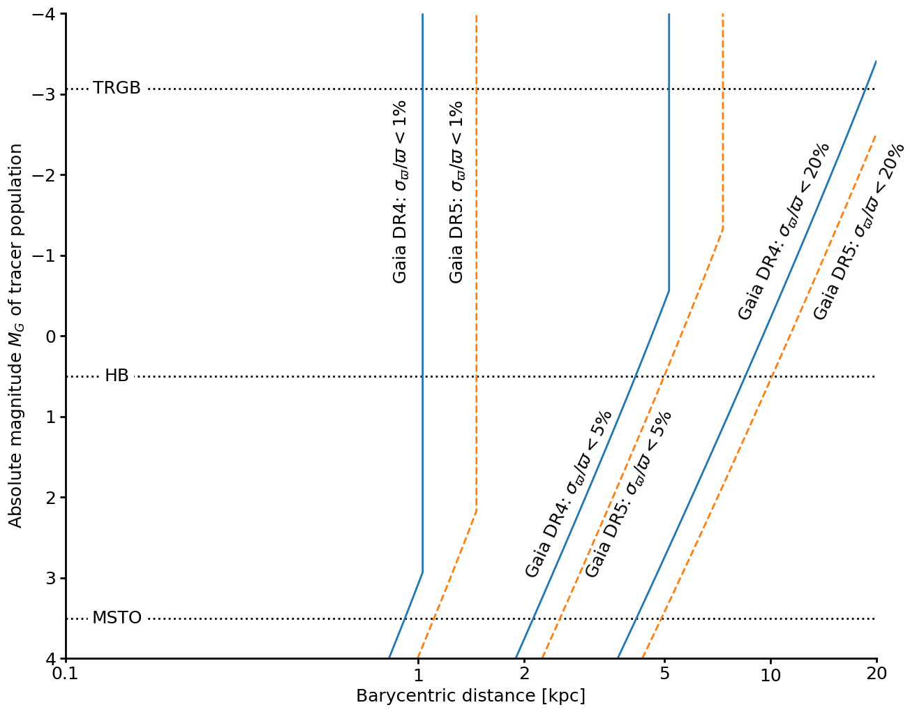
Relative parallax uncertainty horizons#
rhel_plx = np.logspace(np.log10(100), np.log10(20000), 1000)
mabsg, r_plx = np.meshgrid(gabs, rhel_plx)
mg_plx = mabsg + 5 * np.log10(r_plx) - 5
plx_unc_dr4 = parallax_uncertainty(mg_plx, release="dr4")
plx_unc_dr5 = parallax_uncertainty(mg_plx, release="dr5")
rel_plx_unc_dr4 = plx_unc_dr4 * r_plx / 1.0e6
rel_plx_unc_dr5 = plx_unc_dr5 * r_plx / 1.0e6

indices = np.where(mg_plx > 20.7)
rel_plx_unc_dr4[indices] = np.nan
rel_plx_unc_dr5[indices] = np.nan

fig, axplx = plt.subplots(1, 1, figsize=(15, 12))

for y in [gabs_trgb, gabs_hb, gabs_msto]:
    axplx.plot(
        [rhel_plx.min() / 1000, rhel_plx.max() / 1000],
        [y, y],
        lw=2,
        ls="dotted",
        color="k",
        zorder=-1,
    )
axplx.contour(
    rhel_plx / 1000,
    gabs,
    rel_plx_unc_dr4.T,
    levels=[0.01, 0.05, 0.2],
    colors=colors.to_rgba_array(cm.tab10.colors[0]),
    linestyles=["solid"],
)
axplx.contour(
    rhel_plx / 1000,
    gabs,
    rel_plx_unc_dr5.T,
    levels=[0.01, 0.05, 0.2],
    colors=colors.to_rgba_array(cm.tab10.colors[1]),
    linestyles=["dashed"],
)
axplx.invert_yaxis()
axplx.set_xscale("log")
axplx.set_xticks([1, 10], minor=False)
axplx.set_xticklabels(["1", "10"], minor=False)
axplx.set_xticks([0.1, 1, 2, 5, 10, 20], minor=True)
axplx.set_xticklabels(["0.1", "1", "2", "5", "10", "20"], minor=True)
axplx.set_xlabel(r"Barycentric distance [kpc]")
axplx.set_ylabel(r"Absolute magnitude $M_G$ of tracer population")
axplx.text(
    0.14, gabs_msto, "MSTO", ha="center", va="center", bbox=dict(facecolor="w", ec="w")
)
axplx.text(
    0.14, gabs_hb, "HB", ha="center", va="center", bbox=dict(facecolor="w", ec="w")
)
axplx.text(
    0.14, gabs_trgb, "TRGB", ha="center", va="center", bbox=dict(facecolor="w", ec="w")
)

axplx.text(0.9, -0.7, r"Gaia DR4: $\sigma_\varpi/\varpi<1$%", ha="center", rotation=90)
axplx.text(1.3, -0.7, r"Gaia DR5: $\sigma_\varpi/\varpi<1$%", ha="center", rotation=90)
axplx.text(2.7, 3, r"Gaia DR4: $\sigma_\varpi/\varpi<5$%", ha="center", rotation=65)
axplx.text(4, 3, r"Gaia DR5: $\sigma_\varpi/\varpi<5$%", ha="center", rotation=65)
axplx.text(11, -0.2, r"Gaia DR4: $\sigma_\varpi/\varpi<20$%", ha="center", rotation=65)
axplx.text(18, -0.2, r"Gaia DR5: $\sigma_\varpi/\varpi<20$%", ha="center", rotation=65)

plt.show()